(Notebooks and other code available at: https://github.com/csdurfee/hot_hand. As usual, there is stuff in there I'm not covering here.)
What is "approximately normal"?
In the last installment, I looked at NBA game-level player data, which involve very small samples.
Like a lot of things in statistics, the Wald Wolfowitz test says that the number of streaks is approximately normal. What does that mean in practical terms? How approximately are we talking?
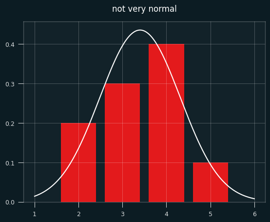
The number of streaks is a discrete value (0,1,2,3,...). In a small sample like 2 makes and 3 misses, which will be extremely common in player game level shooting data, how could that be approximately normal?
Below is a bar chart of the exact probabilities of each number of streaks, overlaid with the normal approximation in white. Not very normal, is it?
To make things more interesting, let's say the player made 7 shots and missed 4. That's enough for the graph to look more like a proper bell curve.
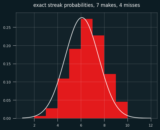
The bell curve looks skewed relative to the histogram, right? That's what happens when you model a discrete distribution (the number of streaks) with a continuous one -- the normal distribution.
A continuous distribution has zero probability at any single point, so we calculate the area under the curve between a range of values. The bar for exactly 7 streaks should line up with the probability of between 6.5 and 7.5 streaks in the normal approximation. The curve should be going through the middle of each bar, not the left edge.
We need to shift the curve to the right a half a streak for things to line up. Fixing this is called continuity correction.
Here's the same graph with the continuity correction applied:
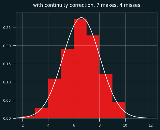
So... better, but there's still a problem. The normal approximation will assign a nonzero probability to impossible things. In this case of 7 makes and 4 misses, the minimum possible number of streaks is 2 and the max is 9 (alternate wins and losses till you run out of losses, then have a string of wins at the end.)
Yet the normal approximation says there's a nonzero chance of -1, 10, or even a million streaks. The odds are tiny, but the normal distribution never ends. These differences go away with big sample sizes, but they may be worth worrying about for small sample sizes.
Is that interfering with my results? It's quite possible. I'm trying to use the mean and the standard deviation to decide how "weird" each player is in the form of a z score. The z score gives the likelihood of the data happening by chance, given certain assumptions. If the assumptions don't hold, the z score, and using it to interpret how weird things are, is suspect.
Exact-ish odds
We can easily calculate the exact odds. In the notebook, I showed how to calculate the odds with brute force -- generate all permutations of seven 1's and four 0's, and measure the number of streaks for each one. That's impractical and silly, since the exact counting formula can be worked out using the rules of combinatorics, as this page nicely shows: https://online.stat.psu.edu/stat415/lesson/21/21.1
In order to compare players with different numbers of makes and misses, we'd want to calculate a percentile value for each one from the exact odds. The percentiles will be based on number of streaks, so 1st percentile would be super streaky, 99th percentile super un-streaky.
Let's say we're looking at the case of 7 makes and 4 misses, and are trying to calculate the percentile value that should go with each number of streaks. Here are the exact odds of each number of streaks:
2    0.006061
3    0.027273
4    0.109091
5    0.190909
6    0.272727
7    0.227273
8    0.121212
9    0.045455
Here are the cumulative odds (the odds of getting that number of streaks or fewer):
2    0.006061
3    0.033333
4    0.142424
5    0.333333
6    0.606061
7    0.833333
8    0.954545
9    1.000000
Let's say we get 6 streaks. Exactly 6 streaks happens 27% of the time. 5 or fewer streaks happens 33% of the time. So we could say 6 streaks is equal to the 33rd percentile, the 33.3%+27.3% = 61st percentile, or some value in between those two numbers.
The obvious way of deciding the percentile rank is to take the average of the upper and lower values, in this case mean(.333, .606) = .47. You could also think of it as taking the probability of streaks <=5 and adding half the probability of streaks=6.
If we want to compare the percentile ranks from the exact odds to Wald-Wolfowitz, we could convert them to an equivalent z score. Or, we can take the z-scores from the Wald Wolfowitz test and convert them to percentiles.
The two are bound to be a little different because the normal approximation is a bell curve, whereas we're getting the percentile rank from a linear interpolation of two values.
Here's an illustration of what I mean. This is a graph of the percentile ranks vs the CDF of the normal approximation.
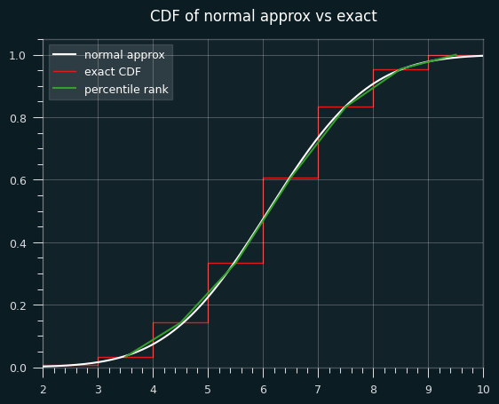
Let's zoom in on the section between 4.5 and 5.5 streaks. Where the white line hits the red line is the percentile estimate we'd get from the z-score (.475).
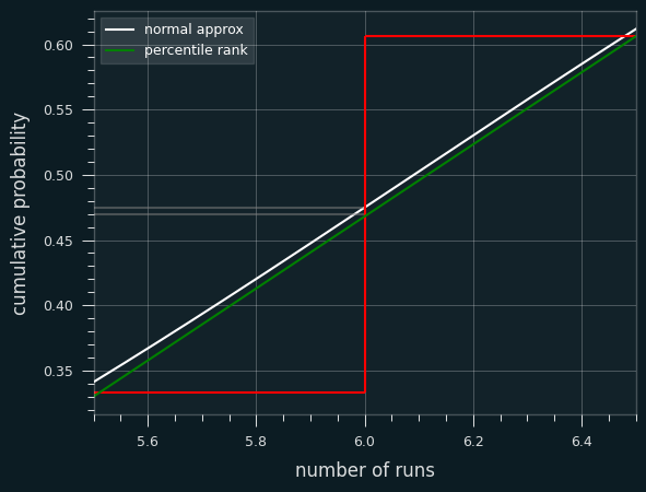
The green line is a straight line that represents calculating the percentile rank. It goes from the middle of the top of the runs <= 5 bar to the middle of the top of the runs <=6 bar. Where it hits the red line is the average of the two, which is percentile rank (.470).
In other situations, the Wald-Wolfowitz estimate will be less than the exact percentile rank. We can see that on the first graph. The green lines and white line are very close to each other, but sometimes the green is higher (like at runs=4), and sometimes the white is higher (like at runs=8).
Is Wald-Wolfowitz unbiased?
Yeah. The test provides the exact expected value of the number of streaks. It's not just a pretty good estimate. It is the (weighted) mean of the exact probabilities.
From the exact odds, the mean of all the streak lengths is 6.0909:
count    330.000000
mean       6.090909
std        1.445329
min        2.000000
25%        5.000000
50%        6.000000
75%        7.000000
max        9.000000
The Wald-Wolfowitz test says the expected value is 1 plus the harmonic mean of 7 and 4, which is 6.0909... on the nose.
Is the normal approximation throwing off my results?
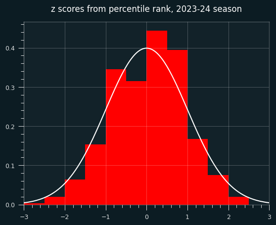
Quite possibly. So I went back and calculated the percentile ranks for every player-game combo over the course of the season.
Here's a scatter plot of the two ways to calculate the percentile on actual NBA player games. The dots above the x=y line are where the Wald-Wolfowitz percentile is bigger than the percentile rank one.
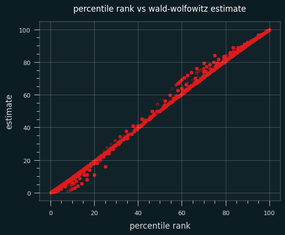
59% of the time, the Wald-Wolfowitz estimate produces a higher percentile value than the percentile rank. The same trend occurs if I restrict the data set to only high volume shooters (more than 10 makes or misses on the game).
Here's a bar chart of the differences between the W-W percentile and the percentile rank:
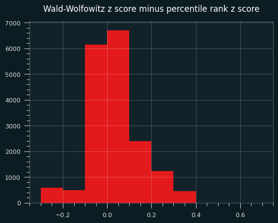
A percentile over 50, or a positive z score, means more streaks than average, thus less streaky than average. In other words, on this specific data set, the Wald-Wolfowitz z-scores will be more un-streaky compared to the exact probabilities.
Interlude: our un-streaky king
For the record, the un-streakiest NBA game of the 2023-24 season was by Dejounte Murray on 4/9/2024. My dude went 12 for 31 and managed 25 streaks, the most possible for that number of makes and misses, by virtue of never making 2 shots in a row.
It was a crazy game all around for Murray. A 29-13-13 triple double with 4 steals, and a Kobe-esque 29 points on 31 shots. He could've gotten more, too. The game went to double overtime, and he missed his last 4 in a row. If he had made the 2nd and the 4th of those, he could've gotten 4 more streaks on the game.
The summary of the game doesn't mention this exceptional achievement. Of course they wouldn't. There's no clue of it in the box score. You couldn't bet on it. Why would anyone notice?
Look at that unstreakiness. Isn't it beautiful?
makes                                                  12
misses                                                 19
total_streaks                                          25
raw_data                  LWLWLWLWLWLWLLWLLLWLWLWLWLWLLLL
expected_streaks                                15.709677
variance                                         6.722164
z_score                                          3.583243
exact_percentile_rank                           99.993423
z_from_percentile_rank                           3.823544
ww_percentile                                   99.983032
On the other end, the streakiest performance of the year belonged to Jabari Walker of the Portland Trail Blazers. Made his first 6 shots in a row, then missed his last 8 in a row.
makes                                  6
misses                                 8
total_streaks                          2
raw_data                  WWWWWWLLLLLLLL
expected_streaks                7.857143
variance                        3.089482
z_score                        -3.332292
exact_percentile_rank             0.0333
z_from_percentile_rank         -3.403206
ww_percentile                   0.043067
Actual player performances
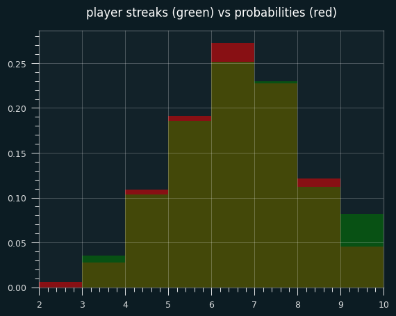
Let's look at actual NBA games where a player had exactly 7 makes and 4 misses. (We can also include the flip side, 4 makes and 7 misses, because it will be the same distribution of streak lengths)
The green areas are where the players had more streaks than the exact probabilities; the red areas are where players had fewer streaks. The two are very close, except for a lot more games with 9 streaks in the player data, and fewer 6 streak games.
The exact mean is 6.09 streaks. The mean for player performances is 6.20 streaks. Even in this little slice of data, there's a slight tendency towards unstreakiness.
Percentile ranks are still unstreaky, though
Well, for all that windup, the game-level percentile ranks didn't turn out all that different when I calcualted them for all 18,000+ player-game combos. The mean and median are still shifted to the un-streaky side, to a significant degree.
Plotting the deciles shows an interesting tendency: a lot more values in the 60-70th percentile range than expected. the shift to the un-streaky side comes pretty much from these values.
![]()
The bias towards the unstreaky side is still there, and still significant:
count    18982.000000
mean         0.039683
std          0.893720
min         -3.403206
25%         -0.643522
50%          0.059717
75%          0.674490
max          3.823544
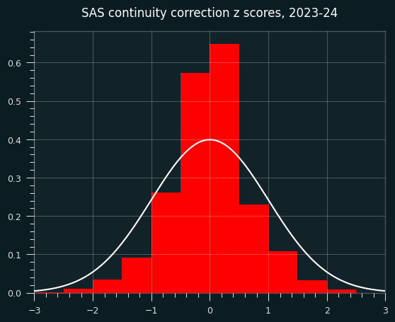
A weird continuity correction that seems obviously bad
SAS, the granddaddy of statistics software, applies a continuity correction to the runs test whenever the count is less than 50.
While it's true that we should be careful with normal approximations and small sample size, this ain't the way.
The exact code used is here: https://support.sas.com/kb/33/092.html
        if N GE 50 then Z = (Runs - mu) / sigma;
        else if Runs-mu LT 0 then Z = (Runs-mu+0.5)/sigma;
          else Z = (Runs-mu-0.5)/sigma;
Other implementations I looked at, like the one in R's randtests package, don't do the correction.
What does this sort of correction look like?
For starters, it gives us something that doesn't look like a z score. The std is way too small.
count    18982.000000
mean        -0.031954
std          0.687916
min         -3.047828
25%         -0.401101
50%          0.000000
75%          0.302765
max          3.390395
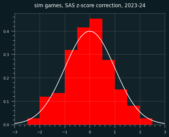
What does this look like on random data?
It could just be this dataset, though. I will generate a fake season of data like in the last installment, but the players will have no unstreaky/streaky tendencies. They will behave like a coin flip, weighted to their season FG%. So the results should be distributed like we expect z scores to be (mean=0, std=1)
Here are the z-scores. They're not obviously bad, but the center is a bit higher than it should be.
However, the continuity correction especially stands out when looking at small sample sizes (in this case, simulated players with fewer than 30 shooting streaks over the course of the season).
In the below graph, red are the SAS corrected z-scores, green are the wald-wolfowitz z scores, brown are the overlap.
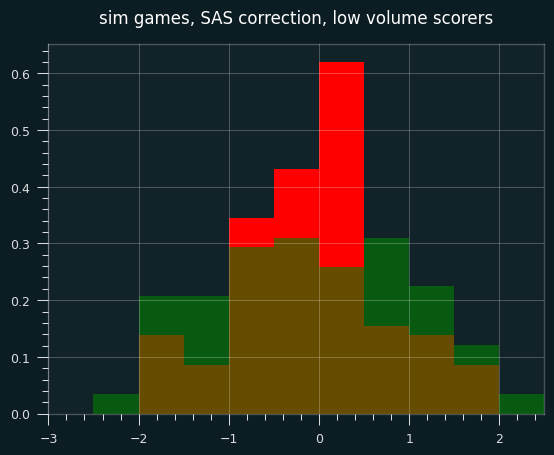
Continuity corrections are at best an imperfect substitute for calculating the exact odds. These days, there's no reason not to use exact odds for smaller sample sizes. Even though it ended up not mattering much, I should've started with the percentile rank for individual games. However, I don't think that the game level results are as important to the case I'm making as the career-long shooting results.
Next time, I will look at the past 20 years of NBA data. Who is the un-streakiest player of all time?